Although the present documentation is not intended as an SQL tutorial, it is useful to provide a chapter about the supported SQL statements.
Most of the statements supported by Ovrimos are standard SQL2 (or SQL/92) statements. There are a few, however, such as CREATE USER, etc. that are SQL-like, but do not belong to the 'body' of SQL.
Conventions of this chapter
All SQL statements and functions, as well as SQL reserved words are CAPITALIZED. They
are written in bold when they appear for the first time and when
the statement syntax is described. Ovrimos SQL, is not case sensitive.
Examples are written in teletype fonts.
time and timestamp have an optional precision, signifying fractional seconds.
time = time(0)
timestamp = timestamp(0)
expression ::=
numeric_expression | float_expression | integer_expression |
string_expression | long_expression | date_expression |
time_expression | timestamp_expression
DATE, TIME and TIMESTAMP are defined and used according to the SQL2 Standard.
Thus, the format for DATE is yyyy-mm-dd.
Whenever DATE is used in an SQL statement, its value must be
enclosed in single quotes (') and preceded by the reserved word DATE.
Thus, the 2nd of December of the year 1962 is described as:
DATE '1962-12-02'.
Legal dates range from '0001-01-01' to '9999-12-31'.
The format of TIME is hh:mm:ss or hh:mm:ss.tttttt (with the .tttttt part,
signifying fractional seconds, optional). Whenever TIME
is used in an SQL statement,
its value must be enclosed in single quotes (') and preceded by the reserved word
TIME.
Thus, 9.30 a.m. is described as:
TIME '09:30:00' or '09:30:00.000000'.
Legal times range from '00:00:00.000000' to '23:59:59.999999'.
It is possible to completely omit the last part (0 digits), but it
is also permitted to have from 1 to 6 digits in the time format. Thus, time:
TIME '09:30:15.50' is legal.
The TIMESTAMP is the DATE and TIME combined, with an optional time zone interval in the form of +hh:mm. The TIME part has an optional fractional seconds part (as TIME).
Whenever used in an SQL statement, the timestamp expression must be enclosed in single quotes (') and preceded by the reserved word TIMESTAMP. The time interval is the time difference of a place from the UTC (Universal Coordinated Time), also known as GMT.
For example, the interval for Athens, Greece is +02:00 and the timestamp for the
11th of September of 1998, at 7.30 PM in Athens is:
TIMESTAMP '1998-09-11 19:30:00+02:00'.
If the timestamp interval is not explicitly set, then the local time zone (i.e. the server time zone is used.) The user may modify the local time zone through the statement SET TIME ZONE. See also, B.4.2.(Supported SQL Statements: Set Time Zone).
The following identifiers are reserved words in Ovrimos SQL.
NOTE: Emphasized keywords are listed as not reserved in SQL2, but
since this is not very meaningful, they are reserved in Ovrimos SQL.
ABSOLUTE, ACTION, ADD, ALL, ALLOCATE, ALTER, AND, ANY, ARE, AS, ASC, ASSERTION, AT, AUTHORIZATION, AVG.
BEGIN, BETWEEN, BIT, BIT_LENGTH, BOTH, BY.
CASCADE, CASCADED, CASE, CAST, CATALOG, CHAR, CHARACTER, CHAR_LENGTH, CHARACTER_LENGTH, CHECK, CLOSE, COALESCE, COLLATE, COLLATION, COLUMN, COMMIT, COMMITTED, CONNECT, CONNECTION, CONSTRAINT, CONSTRAINTS, CONTINUE, CONVERT, CORRESPONDING, COUNT, CREATE, CROSS, CURRENT, CURRENT_DATE, CURRENT_TIME, CURRENT_TIMESTAMP, CURRENT_USER, CURSOR.
DATE, DEALLOCATE, DAY, DEC, DECIMAL, DECLARE, DEFUALT, DEFERRABLE, DEFERRED, DELETE, DESC, DESCRIBE, DESCRIPTOR, DIAGNOSTICS, DISCONNECT, DISTINCT, DOMAIN, DOUBLE, DROP.
ELSE, END, END-EXEC, ESCAPE, EXCEPT, EXCEPTION, EXEC, EXECUTE, EXISTS, EXTERNAL, EXTRACT.
FALSE, FETCH, FIRST, FLOAT, FOR, FOREIGN, FOUND, FROM, FULL.
GET, GLOBAL, GO, GOTO, GRANT, GROUP.
HAVING, HOUR.
IDENTITY, IMMEDIATE, IN, INDICATOR, INITIALLY, INNER, INPUT, INSENSITIVE, INSERT, INT, INTEGER, INTERSECT, INTERVAL, INTO, IS, ISOLATION.
JOIN
KEY
LANGUAGE, LAST, LEADING, LEFT, LEVEL, LIKE, LOCAL, LOWER
MATCH, MAX, MIN, MINUTE, MODULE, MONTH
NAMES, NATIONAL, NATURAL, NCHAR, NEXT, NO, NOT, NULL, NULLIF, NUMERIC
OCTET_LENGTH, OF, ON, ONLY, OPEN, OPTION, OR, ORDER, OUTER, OUTPUT, OVERLAPS
PARTIAL, POSITION, PRECISION, PREPARE, PRESERVER, PRIMARY, PRIOR, PRIVILEGES, PROCEDURE, PUBLIC
QUIT
READ, REAL, REFERENCES, RELATIVE, RESTRICT, REVOKE, REPEATABLE, RIGHT, ROLLBACK, ROWS
SCHEMA, SCROLL, SECOND, SECTION, SELECT, SESSION, SESSION_USER, SERIALIZABLE, SET, SIZE, SMALLINT, SOME, SQL, SQLCODE, SQLERROR, SQLSTATE, SUBSTRING, SUM, SYSTEM_USER
TABLE, TEMPORARY, THEN, TIME, TIMESTAMP, TIMEZONE_HOUR, TIMEZONE_MINUTE, TO, TRAILING, TRANSACTION, TRANSLATE, TRANSLATION, TRIM, TRUE, TYPE
UNCOMMITTED, UNION, UNIQUE, UNKNOWN, UPDATE, UPPER, USAGE, USER, USING, VALUE, VALUES, VARCHAR, VARYING, VIEW
WHEN, WHENEVER, WHERE, WITH, WORK, WRITE
YEAR
ZONE
Additional ODBC 2.0 SQL Keywords:
BIGINT, BINARY, TINYINT, VARBINARY
Additional Ovrimos SQL Keywords:
CALL, FIND_COLUMN, FUNCTION, INDEX, UNICODE, UNSIGNED
A demonstration database , testbase , is provided, to help users familiarize themselves with Ovrimos features. See 2.3.1.(Populating testbase), for setting up testbase. For better understanding of the examples, the contents of some sample tables are presented here. All these tables may be found in testbase after populating it with sample data.
Name |
Descr | S | Distance | Small_pic | Big_pic |
Mercury |
The planet where days last longer than years | 1 | 36.0 | image/gif | image/jpeg |
| Venus | The greenhouse planet | 2 | 67.1 | image/gif | image/jpeg |
| Earth | Mostly harmless | 3 | 92.7 | image/gif | image/jpeg |
| Mars | The red planet | 4 | 141.5 | image/gif | image/jpeg |
| Jupiter | The sun that failed | 5 | 483.4 | image/gif | image/jpeg |
| Saturn | The ringed planet | 6 | 886.7 | image/gif | image/jpeg |
| Uranus | The rolling planet | 7 | 1782.7 | image/gif | image/jpeg |
| Neptune | The blue planet | 8 | 2794.0 | image/gif | image/jpeg |
| Pluto | The paired planet | 9 | 3666.1 | image/gif | image/jpeg |
| Name | Planet | Small_pic | Big_pic |
| Moon | Earth | image/gif | image/jpeg |
| Phobos | Mars | image/gif | image/jpeg |
| Deimos | Mars | image/gif | image/jpeg |
| Callisto | Jupiter | image/gif | image/jpeg |
| Ganymede | Jupiter | image/gif | image/jpeg |
| Io | Jupiter | image/gif | image/jpeg |
| Europa | Jupiter | image/gif | image/jpeg |
| Enceladus | Saturn | image/gif | image/jpeg |
| Dione | Saturn | image/gif | image/jpeg |
| Titan | Saturn | image/gif | image/jpeg |
| Tethys | Saturn | image/gif | image/jpeg |
| Rhea | Saturn | image/gif | image/jpeg |
| Mimas | Saturn | image/gif | image/jpeg |
| Oberon | Uranus | image/gif | image/jpeg |
| Titania | Uranus | image/gif | image/jpeg |
| Umbriel | Uranus | image/gif | image/jpeg |
| Triton | Neptune | image/gif | image/jpeg |
| Charon | Pluto | image/gif | image/jpeg |
Columns Small_pic and Big_pic are .gif and .jpg images respectively. In the table columns these are links to a place containing the image. See B.9.(BLOBs and the URI function).
Tables Customers, Salespeople, and Orders contain data on a sales system.
| Cid | Cname | City | Rating | Sid |
| 2001 | Hanson | Helsinki | 100 | 1001 |
| 2002 | Gerard | Athens | 200 | 1003 |
| 2003 | Longman | Rome | 200 | 1002 |
| 2004 | Gable | London | 300 | 1002 |
| 2006 | Conrad | Helsinki | 100 | 1001 |
| 2007 | Carlton | Paris | 300 | 1007 |
| 2008 | Peterson | New York | 100 | 1004 |
| Sid | Sname | City | Commission |
| 1001 | Pelee | Helsinki | 0.11 |
| 1002 | Sarmani | Rome | 0.12 |
| 1004 | Moss | Helsinki | 0.13 |
| 1007 | Randall | Paris | 0.09 |
| 1003 | Anakin | New York | 0.12 |
| Ordid | Quantity | Odate | Cid | Sid |
| 3001 | 25 | 1998-12-22 | 2008 | 1007 |
| 3002 | 38 | 1998-12-23 | 2007 | 1001 |
| 3003 | 129 | 1998-12-23 | 2001 | 1004 |
| 3004 | 72 | 1999-01-04 | 2004 | 1002 |
| 3005 | 18 | 1999-01-04 | 2002 | 1007 |
| 3006 | 31 | 1999-01-05 | 2006 | 1003 |
| 3007 | 55 | 1999-01-07 | 2004 | 1001 |
| 3008 | 62 | 1999-01-07 | 2003 | 1002 |
Table Orders is later altered during the course of an example. A new column ordtime of type TIME is added. The column is originally NULL. When the rows are added, data are inserted into the new column ordtime, but only in the new rows.
| ISBN | TITLE | AUTHOR | PRICE | COVER |
| 999-4444-22-1 | 50 ways to feed a cat | D. H. Hackleberry | 12.50 | image/gif |
| 999-4434-21-1 | Ancient Egypt | D. H. Hackleberry | 35.00 | image/gif |
| 989-2444-22-9 | What I saw in Congo | Apple J. Pie | 34.00 | image/gif |
| 499-4144-52-8 | Teach yourself Cobol in 21 days | Egbert H. Cailloux | 34.50 | image/gif |
| 499-6447-12-4 | Surfing USA | D. Boy | 45.00 | image/gif |
Finally, there is a table called uni, used for examples of unicode insertion and retrieval.
| Initial_char | Uni_symbols |
This table is empty. If you wish to fill-in sample data, look at the examples in B.10.(Storage and Retrieval of Unicode Data) .
At some point, a user pandora and a user friend are added to the database.
Alter Table
Create Domain
Create Index
Create Table
Create User
Create View
Drop Domain
Drop Index
Drop Table
Drop User
Drop View
Delete Positioned
Update Positioned
Set Transaction
Commit
Rollback
Grant
Revoke
column_definition ::=
column_name {domain_name| data_type }
[column_constraint ...]
[DEFAULT default value];
and
column_constraint ::=
PRIMARY KEY | REFERENCES table_name [(column_name_list)]
| NOT NULL | UNIQUE | CHECK (expression)
Each statement is followed by a short description text, the statement syntax and a short example.
SQL Syntax:
ALTER TABLE table name ADD column_definition;
or
ODBC Syntax:
ALTER TABLE table name ADD (column_definition_list);
See B.4.1.(column_definition_list) for details of column definition.
Example:
ALTER TABLE orders ADD Ordtime TIME;
So, if the table was:
| Ordid | Quantity | Odate | Cid | Sid |
The altered table will be:
| Ordid | Quantity | Odate | Cid | Sid | Ordtime |
Note: Only ADD is permitted in ALTER TABLE.
Syntax:
CALL proc-name [arguments]
Example:
CALL insert_data
where insert_data is a stored procedure.
Syntax:
CREATE DOMAIN domain_name [AS] data type
[constraint_definition]
where
constraint_definition ::= conditional_expression;
See more about constraints in B.4.1.(Definition Grammar).
Example:
CREATE DOMAIN nat_number integer
check value > 0;
Inside the conditional_expression the special identifier value denotes the value being checked.
The newly created domain nat_number will be used in Data Definition (usually when creating a table) as an integer number greater than 0, i.e. as a natural number.
Syntax:
CREATE [UNIQUE] INDEX index_name ON table_name
(column_name [ASC|DESC].,...);
Example:
CREATE UNIQUE INDEX ind1 ON planets (Serial ASC);
The new index ind1, will be used as an index in ascending order.
Its values must be unique.
Note: This is not a standard SQL statement, although it's quite common.
Syntax:
CREATE TABLE table_name
({column_definition|[table_constraint]},...)
where
table_constraint ::=
PRIMARY KEY (column_name_list)
| FOREIGN KEY (column_name_list)
REFERENCES table_name [(column_name_list)]
| CHECK (expression)
| UNIQUE (column_name_list)
For a detailed description of column_definition see B.4.1.(column_definition_list).
Example:
CREATE TABLE Planets (
Name varchar(15) PRIMARY KEY,
Descr varchar(50),
Serial_number nat_number UNIQUE,
Distance_mmiles decimal(5,1),
Small_pic long varbinary,
Big_pic long varbinary
);
The newly created table Planets was presented in the beginning of this chapter.
Similarly, one can see another example of table creation, where foreign keys also exist, in the definition of table Satellites, which is also presented in the beginning of the chapter.
Example:
CREATE TABLE Satellites (
Name varchar(15) PRIMARY KEY,
Planet varchar(15) REFERENCES Planets(name),
Small_pic long varbinary,
Big_pic long varbinary
);
Syntax:
CREATE USER username FOR 'full-user-name'
WITH 'password'| NULL
[LIKE prototype user]
[USING 'attribute=value;attribute=value...'];
where
attribute::=REMARKS | MAILBOX
Users with NULL password may not login.
The attribute remarks is only a string that appears next to the user description and has no other use. Attribute mailbox however, contains the mail address of a particular user. This address may be a simple user name (if the mailbox resides in $MAILSERVER) or a full mailbox otherwise. See also, A.2.2.(Database Parameters).
The mailbox attribute appears next to the user description in Roadmap. It may be used by admin to send mail to a user. It is also used by Ovrimos to inform admin of unsuccessful logins. See 13.4.3.(Unauthorized Logins).
Example:
CREATE USER pandora FOR 'Mary Adams'
WITH 'pass1' LIKE admin;
This statement will create a user with name pandora and initial password pass1. This new user is like admin, which means she has full privileges. This is an example of privilege inheritance.
Example:
CREATE USER friend FOR 'Joe Phillips'
WITH 'pass2';
This user has no admin privileges.
Example:
CREATE USER Farad FOR 'John Faraday' WITH 'pass3'
USING 'mailbox=jfar';
A mailbox address, set in a local network mailserver, is set for user Farad.
Note! Users who communicate with a secure database are required to have a mail address if the authorization is done via certificates. The mailbox must be the same as the one given for the client's certificate. If authorization is checked only through passwords, the mailbox is not necessary.
For more information about passwords see 13.4.2.(Password Policy).
Note: This is not a standard SQL statement.
Syntax:
CREATE VIEW table name [(column_list)]
AS SELECT statement;
Example:
CREATE VIEW Planet_list
AS SELECT Name, Descr FROM planets
WHERE Serial >= 5;
The Create View statement will make a view called planet_list, where only two columns of Planets will be visible. For users of planet_list the view will appear like:
Planet_list
| Name | Descr |
| Jupiter | The sun that failed |
| Saturn | The ringed planet |
| Uranus | The rolling planet |
| Neptune | The blue planet |
| Pluto | The paired planet |
All views have CASCADED CHECK OPTION as default.
The CHECK OPTION does not allow users to insert into the view or update rows to values that violate view constraints. For example, if a view is created as:
CREATE VIEW outer_planets
AS SELECT * FROM planets
WHERE Serial > 4;
it is not allowed to insert a row where Serial <= 4.
Should you be allowed to insert such a row, then because of the existing view constraint (set at creation time), you would not be able to retrieve this row!
Following the same line of thought, CASCADED CHECK OPTION, means that new views based on this view, 'inherit' the CHECK of the base view. Thus, if we have a view created as:
CREATE VIEW gas_planets
AS SELECT * FROM outer_planets
WHERE ...;
this new view, besides all its other constraints, will also check the constraint of Serial > 4, set by the base view.
Syntax:
DELETE FROM table name
WHERE CURRENT OF cursor name;
Example:
DELETE FROM planets WHERE CURRENT OF Cur1;
The cursor Cur1 is previously defined to traverse the table. The cursor is positioned to a certain row, usually after the execution of a select statement. The statement will delete the row where the cursor is positioned. After deletion of the row, the position of the cursor is undefined.
Syntax:
DELETE FROM table name [WHERE predicate];
Example:
DELETE FROM planets WHERE Distance_mmiles > 3000;
This statement will delete the rows (if any), where the planet distance is greater than 3000 million miles. In our example, Pluto will be removed from the table.
Warning! Do not use the DELETE statement to remove users from the database. It may prove detrimental! Use the provided Drop User instead.
Syntax:
DROP DOMAIN domain_name;
Example:
DROP DOMAIN nat_number;
After the Drop Domain statement, the identifier nat_number may no longer be used as a data type. The columns of tables already defined by this domain are not affected from the domain deletion, since the domain is used as a macro, which is expanded at the time of column definition and does not appear anywhere else.
Syntax:
DROP INDEX index name;
Example:
DROP INDEX ind1;
After the Drop Index statement, the columns involved in the ind1 index are no longer used as a key. If the index was defined as UNIQUE, the constraint, that was checked during insertion or update on columns participating in the index, is no longer checked.
Note: This is not a standard SQL statement.
Syntax:
DROP TABLE table name [CASCADE|RESTRICT];
The option RESTRICT is the default. If CASCADE is specified, then, when a table is removed all its dependent views are also removed. The option RESTRICT does not allow table removal when it has dependent views.
Example:
DROP TABLE planets;
The table planets is removed and all its data are deleted. Since no option is explicitly stated, any views dependent on it (such as planet_list) are also dropped. Foreign keys constraints are also dropped.
Syntax:
DROP USER user name;
Example:
DROP USER friend;
After the statement, user friend is no longer in the system. All tables and views created by user friend are now owned by user admin, who may decide to grant privilege to some other user for management and data manipulation of these tables.
Note: This is not a standard SQL statement.
Syntax:
DROP VIEW view name [CASCADE|RESTRICT];
The option CASCADE is the default. When a view is removed all its dependent views are also removed. The option RESTRICT does not allow view removal when it has dependent views.
Example:
DROP VIEW outer_planets;
The view outer_planets is removed and all its data are deleted. Since no option is explicitly stated, any views dependent on it are also dropped.
Syntax:
GRANT privilege,... ON object_name
TO {grantee,...}|PUBLIC
[WITH GRANT OPTION];
where
privilege::=
{ALL PRIVILEGES} |
{SELECT
| DELETE
| {INSERT [(column name,...)]}
| {UPDATE [(column name,...)]}
| {REFERENCES [column name,...)]}
}
object_name::= [TABLE] table_name
and
table_name ::= base_table_name | view_name
Two examples about granting privileges follow:
Example:
GRANT ALL PRIVILEGES ON planets TO pandora;
GRANT SELECT, INSERT ON satellites TO pandora
with GRANT OPTION;
The first statement allows full privileges to user pandora on table Planets. The second allows SELECT and INSERT to user pandora on table Satellites. The GRANT OPTION allows the user to pass this privilege to other users as well.
We must note at this point, that granting privileges to a view grants automatically privileges to the base table. This is not the standard SQL treatment of privileges.
Syntax:
INSERT INTO table_name [(column name,...)]
query_expression|table_value_constructor;
where
table_value_constructor ::= VALUES (value, ...)
A detailed description of query_expression may be found in B.4.1.(Definition Grammar).
Example:
INSERT INTO Planets (Name, Descr, Serial)
VALUES ('Mercury','The planet where days last longer than years', 1);
Warning! Do not use the INSERT statement to directly add users to the database. It may prove detrimental! Use the provided Create User instead.
Syntax:
REVOKE [GRANT OPTION FOR]
{ALL PRIVILEGES} | {privilege,...}
ON object_name
FROM PUBLIC | {grantee,...};
Two example about revoking privileges follow:
Example:
REVOKE INSERT, DELETE ON Planets FROM pandora;
REVOKE GRANT OPTION FOR
SELECT ON Satellites FROM pandora;
The first statement revokes the INSERT and DELETE option from user pandora, while the second disallows user pandora to grant the SELECT option to other users. (User pandora retains her privilege to SELECT from Satellites.)
Syntax:
query_expression
[UNION[ALL] select_statement | TABLE table_name
[ORDER BY {{output_column [ASC|DESC]},...}
| {{positive integer [ASC|DESC]},...}];
The first part of the Select syntax is query_expression, which is described in detail in B.4.1.(Definition Grammar).
Example:
SELECT Descr FROM Planets WHERE Name = 'Earth';
| Descr |
| Mostly harmless |
Example:
SELECT count(*) FROM planets
WHERE Distance_mmile > 100;
| count |
| 6 |
The following example is a SELECT with a subquery, where the two tables are connected with the matching name of the planet.
Example:
SELECT Planets.Name, Descr FROM planets
WHERE Name = (SELECT Planet FROM Satellites
WHERE Satellites.Name = 'Titania');
| Name | Descr |
| Uranus | The rolling planet |
The following example will return the planets ordered by decreasing distance.
Example:
SELECT Name FROM planets ORDER BY distance_mmiles DESC;
| Name |
| Pluto |
| Neptune |
| Uranus |
| Saturn |
| Jupiter |
| Mars |
| Earth |
| Venus |
| Mercury |
The following SELECT statement joins the tables Planets and Satellites and produces a sequence of rows with all planets and satellites that have Serial less than 6. Thus, Saturn, Uranus, Neptune and Pluto are not included in the output.
Example:
SELECT planets.name, satellites.name
FROM planets, satellites
WHERE planets.name = satellites.planet
AND serial < 6;
| Name | Name |
| Earth | Moon |
| Mars | Phobos |
| Mars | Deimos |
| Jupiter | Io |
| Jupiter | Europa |
| Jupiter | Ganymede |
| Jupiter | Callisto |
A few more Select examples based on the Customers, Salespeople and
Orders sample tables follow, to show how complex queries may be written in SQL.
Select within a select
Example:
SELECT * FROM Orders
WHERE Sid IN
(SELECT Sid FROM Salespeople WHERE City = 'Helsinki');
| Ordid | Quantity | Odate | Cid | Sid |
| 3003 | 129 | 1998-12-23 | 2001 | 1004 |
| 3007 | 55 | 1999-01-07 | 2004 | 1001 |
Select with implicit table join
Example:
SELECT Customers.Cname, Salespeople.Sname, Salespeople.City
FROM Salespeople, Customers
WHERE Salespeople.City = Customers.City;
This query returns the names of Customers and Salespeople who work in the same city,
as well as the name of the city.
| Cname | Sname | City |
| Hanson | Pelee | Helsinki |
| Conrad | Pelee | Helsinki |
| Longman | Sarmani | Rome |
| Hanson | Moss | Helsinki |
| Conrad | Moss | Helsinki |
| Carlton | Randall | Paris |
| Peterson | Anakin | New York |
Example:
SELECT Customers.Cname, Salespeople.Sname
FROM Customers, Salespeople
WHERE Salespeople.Sid = Customers.Sid;
This query returns the salesperson corresponding to each customer.
| Cname | Sname |
| Hanson | Pelee |
| Conrad | Pelee |
| Longman | Sarmani |
| Gable | Sarmani |
| Peterson | Moss |
| Carlton | Randall |
| Gerard | Anakin |
Select with ANY
Example:
SELECT * FROM Salespeople
WHERE City = ANY (Select CITY FROM Customers)
ORDER BY City;
| Sid | Sname | City | Commission |
| 1001 | Pelee | Helsinki | 0.11 |
| 1004 | Moss | Helsinki | 0.13 |
| 1003 | Anakin | New York | 0.12 |
| 1007 | Randall | Paris | 0.09 |
| 1002 | Sarmani | Rome | 0.12 |
Select with UNION
The following query returns the UNION of Salespeople who work in Helsinki and
of Customers who dwell there.
Example:
SELECT Sid, Sname FROM Salespeople
WHERE City = 'Helsinki'
UNION
SELECT Cid, Cname FROM Customers
WHERE City = 'Helsinki';
| 1001 | Pelee |
| 1004 | Moss |
| 2001 | Hanson |
| 2006 | Conrad |
Notice that there are no headers in the example above, since the returned rows come from different tables.
Syntax:
Select_statement FOR UPDATE OF;
where
select_statement ::=
query_expression
[UNION[ALL] select_statement | TABLE table_name];
A detailed description of query_expression may be found in B.4.1.(Definition Grammar).
Example:
SELECT Distance_mmiles FROM planets
WHERE Serial = 4 FOR UPDATE OF;
This statement sets the cursor to the selected row for a future update. It may not be used directly from an UPDATE statement.
Note also that when a Select for Update is executed, the selected rows are locked for update and they remain locked until the transaction is committed, while a simple Select statement locks the rows only when the Isolation Level is REPEATABLE READ or SERIALIZABLE. See also 13.1.2.(Transaction Atomicity).
When a session starts, the default time zone is the time zone of the server. (Note! Not the local time zone of the computer where the user works, but the local time zone of the computer where Ovrimos resides.)
If the default time zone is not convenient, users may modify their time zone with the SET TIME ZONE statement. This does not affect internal representation of times and timestamps. It only affects the way information will be displayed for the user.
Syntax:
SET TIME ZONE value | LOCAL;
Example:
SET TIME ZONE LOCAL;
The above statement sets the time zone to the local time zone of the server, not the client computer.
Example:
SET TIME ZONE '+02:00';
The above statement sets the time zone to +2 hours of UTC (GMT). Times are always kept in UTC internally, but they are returned as local times (according to the time zone of the session).
Example of time zone usage:
Suppose table Orders is altered (as shown in the Alter Table statement)
and contains now a new column Ordtime. The time zone of the server is set +2 hours
of UTC and a new order is inserted:
Example:
SET TIME ZONE '+02:00';
INSERT INTO Orders VALUES
(3010, 40, DATE '1999-11-11', 2008, 1003, TIME '11:05:00');
This is local time 11:05:00, which corresponds to UTC 09:05:00, since the time zone was set to +2.
Selecting the new order from the table will return the following:
Example:
SELECT * FROM Orders WHERE Ordid = 3010;
| Ordid | Quantity | Odate | Cid | Sid | Ordtime |
| 3010 | 40 | 1999-11-11 | 2008 | 1003 | 11:05:00 |
We may now set the local time to +10 from UTC.
Example:
SET TIME ZONE '+10:00';
The previous SELECT * FROM Orders WHERE Ordid = 3010;
statement will return the following:
| Ordid | Quantity | Odate | Cid | Sid | Ordtime |
| 3010 | 40 | 1999-11-11 | 2008 | 1003 | 19:05:00 |
Of course, the internal representation of the time is not affected by either of the SET
TIME ZONE statement. Internally, the time is UTC, i.e. 09:05:00.
The presentation of columns defined as TIMESTAMPS is similarly affected by the SET TIME ZONE statement.
Syntax:
SET TRANSACTION
{ISOLATION LEVEL
{READ UNCOMMITTED
| READ COMMITTED
| REPEATABLE READ
| SERIALIZABLE}
} | {READ ONLY|READ WRITE}
Example:
SET TRANSACTION ISOLATION LEVEL READ COMMITTED;
The next transaction will be performed on the READ COMMITTED level.
Syntax:
UPDATE table name
SET {column_name = {value_expression | NULL}},...
WHERE CURRENT OF cursor name;
Example:
UPDATE planets SET Distance_mmile = 21000000
WHERE CURRENT OF cur1;
The Distance_mmile field of the row where cursor cur1 has been placed will be updated.
Syntax:
UPDATE table_name
SET {column_name = {value_expression|NULL}},...
[WHERE predicate];
Example:
UPDATE Planets SET Distance_mmile = 21000000
WHERE Serial = 4;
Warning! Do not use the UPDATE statement to modify system tables, such as sys.users etc. It may prove detrimental to your database! Use the provided Update User instead.
Syntax:
UPDATE USER user_name
[WITH 'new password'|NULL]
[LIKE prototype user]
[USING 'attribute=value;attribute=value...'];
where
attribute::= REMARKS | MAILBOX
For explanation of the attributes remarks and mailbox, see the Create User statement in the same section.
Example:
UPDATE USER pandora WITH 'xyzzy';
UPDATE USER friend LIKE pandora;
The first statement changes the password of user pandora, while the second gives the privileges of user pandora to user friend. Of course, the second statement does not affect friend's password.
The following is the statement user admin has to execute to modify
his/her initial password, which (in the beginning) is known to all.
UPDATE USER admin WITH 'new password';
Note! Users who communicate with a secure database are required to have a mail address if the authorization is done via certificates. The mailbox must be the same as the one given for the client's certificate. If authorization is checked only through passwords, the mailbox is not necessary.
Note: This is not a standard SQL statement.
Syntax:
COMMIT [WORK];
Syntax:
ROLLBACK [WORK];
The SQL aggregate functions are described by:
COUNT(*)
all-function::={AVG|MAX|MIN|
SUM} ([ALL] expression)
distinct-function::={AVG|COUNT|MAX|MIN|SUM}
(DISTINCT column-name)
Return values of the aggregate functions:
The result of COUNT(*) is an integer. COUNT(DISTINCT) is also integer.
NULL values found in the query are counted.
When no rows are found complying to the subquery, COUNT returns 0.
MAX and MIN return results of the same type as their input columns.
When no rows are found complying to the subquery, MAX and MIN return NULL.
AVG and SUM return values depending on their inputs:
On tinyint and smallint, they return integer.
On unsigned smallint and unsigned tinyint, they return
unsigned int.
On decimal and numeric, they return
decimal and numeric with precision 15.
For the rest of the input types the aggregate functions have the same types.
When no rows complying to the subquery are found, AVG and SUM return NULL.
Syntax:
CAST ( scalar-expression AS data-type )
Example:
SELECT CAST (4 AS decimal(3,1)) FROM tempo
(where tempo is a temporary table) returns 4.0
Note: Some data types may not be converted to others.
Syntax:
CASE
when-clause-list
ELSE scalar-expression
END
where a 'when-clause' takes the form:
WHEN conditional-expression THEN scalar-expression
Example:
CASE
WHEN value < 100 THEN 'Cheap'
WHEN value < 200 THEN 'Medium'
ELSE 'Expensive'
END
Example:
SELECT user_name, CASE WHEN user_name='ADMIN' THEN 'Administrator'
WHEN user_name='PUBLIC' THEN 'Public'
ELSE 'Other' END
FROM sys.users
This will return all the database users with the classification, 'Administrator',
'Public' or 'Other'.
Similarly, CASE may also be used as follows:
Syntax:
CASE column_name
WHEN value THEN result
...
ELSE scalar-expression END
FROM table_name
Example:
SELECT user_name, CASE user_name
WHEN 'ADMIN' THEN 'A!'
WHEN 'PUBLIC' THEN 'P!' ELSE 'O!' END
FROM sys.users
POSITION (string2 IN string1)
is defined to return a value as follows:
If the CHARACTER_LENGTH of string2 is zero, the result is 1.
Otherwise, if string2 occurs as a substring within string1,
the result is one greater than the number of characters in string1 that precede
the first such occurrence.
Otherwise the result is zero.
Example:
SELECT POSITION ('ha' IN 'Alpha')
FROM tempo
returns 4.
Example:
SELECT SUBSTRING ('Good Morning' FROM 3 FOR 4)
FROM tempo
returns 'od M'.
In general, the string argument can be any character or bit string expression, and the FROM and FOR arguments can be any numeric expression. If FOR is omitted, all the right part from FROM is extracted.
Syntax:
TRIM (ltb pad FROM string)
ltb = LEADING, TRAILING or both.
If omitted, option BOTH is assumed.
<pad> is a character string expression that evaluates to a single character.
The <pad> character to be removed is specified.
If the <pad> character is not specified, then space is assumed.
If <ltb> and <pad> are omitted, FROM must also be omitted.
Example:
INSERT INTO tempo VALUES (USER,...),
causes the user name to be inserted into a row in the table tempo.
CASE WHEN x = y THEN NULL ELSE x END
Example:
SELECT nullif (2+3, 4+1) FROM tempo
returns NULL,
while
SELECT nullif (4+2, 4+1) FROM tempo
returns 6
The expression COALESCE (x, y)
is defined to be equivalent to the expression
CASE WHEN x is NOT NULL THEN x ELSE y END
In general, COALESCE (x,y, ..., z) returns NULL only if all its operands evaluate to NULL.
Ovrimos provides you with a variety of functions, that may be used in combination with the above described SQL statements. Some of these functions comply with ODBC requirements, while a few are implemented to allow BLOB insertion and retrieval.
These functions belong to the following general categories: Mathematical functions, Date and Time functions, String manipulation functions, BLOB reference manipulation functions and System functions.
A brief description of the function, together with the arguments and the return values, is provided below. Several functions are overloaded. The user may also note the underscore (_) in the beginning of some function names. This was used to differentiate functions such as DATE and TIME etc. from reserved SQL words.
All the above mentioned expressions may be literals, results of other scalar functions, names of columns etc.
Table Tempo
| Angle | Number |
Example:
SELECT ABS(number) FROM tempo
returns 3.4 if the number is either 3.4 or -3.4.
Example:
SELECT ACOS (number) FROM tempo
on number 0, returns 1.5707963, i.e. ![]() .
.
Example:
SELECT ASIN (number) FROM tempo
on number 1, returns ![]() .
.
Example:
SELECT ATAN(number) FROM tempo
on number 1, returns 0.785398, i.e. ![]() .
.
Example:
SELECT ATAN2 (Xcoord, Ycoord) FROM tabname
on Xcoord = 10 and Ycoord = 10 returns 0.785398. i.e ![]() .
.
Example:
SELECT CEILING (number) FROM tempo
on number = 5.4 returns 6.
SELECT CEILING (number) FROM tempo
on number = -5.4 returns -5.
Example:
SELECT COS (angle) FROM tempo
on angle 0, returns 1.
Example:
SELECT COT (angle) FROM tempo
on angle pi/4, returns 1.
Example:
SELECT DEGREES (pi()) FROM tempo
returns 180.
Example:
SELECT EXP (number) FROM tempo
on number 4, returns 54.59815, i.e. e4.
Example:
SELECT FLOOR (number) FROM tempo
on number 3.4, returns 3, and on number -3.4, returns -4.
Example:
SELECT LOG (number) FROM tempo
on number e3, returns 3.
Example:
SELECT LOG10 (number) FROM tempo
on number 1000, returns 3.
Example:
SELECT MOD (number,3) FROM temp
on number 20, returns 2.
Example:
UPDATE tempo SET angle = PI()
sets angle to 3.14159...
Example:
SELECT POWER (2,8) FROM tempo
returns 256.
Example:
SELECT RADIANS (90) FROM tempo
returns 1.5707963, i.e. ![]() .
.
Example:
SELECT RAND() FROM tempo
returns a random value.
Example:
SELECT ROUND (number, 2) FROM tempo
on number 7.1278, returns 7.13.
SELECT ROUND (number, -2) FROM tempo
on number 7.1278, returns 0.
Example:
SELECT SIGN (number) FROM tempo
on number 10, returns 1
on number 0, returns 0
on number -10, returns -1
Example:
SELECT SIN (angle) FROM tempo
on number ![]() ,
returns 1.
,
returns 1.
Example:
SELECT SQRT (number) FROM tempo
on number 16, returns 4.
Example:
SELECT TAN (angle) FROM tempo
on number ![]() ,
returns 1.
,
returns 1.
Example:
SELECT TRUNCATE (number, 2) FROM tempo
on number 7.1278 returns 7.12.
SELECT TRUNCATE (number, -2) FROM tempo
on number 7.1278 returns 0.
Example:
CREATE TABLE A (I, int IDENTITY(10,5)
where I is numeric_expression, CHAR or VARCHAR.
IDENTITY(seed, increment)
increments the seed by increment each time it is called.
It is also possible to have IDENTITY with only one argument, A. In this case, IDENTITY returns the last value that was assigned to A.
For making the examples of time and date functions more solid, we assume a table
tempo, with columns date_field, time_field and
tstamp_field of types DATE, TIME and TIMESTAMP respectively.
The following time and date functions do not accept all the types required by ODBC. Specifically, CHAR and VARCHAR are not accepted by these functions.
Example:
EXTRACT (MINUTE FROM TIME '09:30:00')
returns 30.
Example:
SELECT _HOUR (time_field) FROM tempo
on time_field 22:17:21, returns 22.
SELECT _HOUR (TIME '21:18:50') FROM tempo
returns 21.
Example:
SELECT _MINUTE (time_field) FROM tempo
on time_field 22:17:21, returns 17.
Example:
SELECT _MONTH (date_field) FROM tempo
on date_field 1998-10-12, returns 10.
SELECT _MONTH (DATE '1999-02-15') FROM tempo
returns 2.
Example:
SELECT _SECOND (time_field) FROM tempo
on time_field 22:17:21, returns 21.
Example:
SELECT _YEAR (date_field) FROM tempo
on date_field 1998-10-12, returns 1998.
If a statement began at 10:20 am on October 15th 1998, then
Example:
SELECT CURDATE () FROM tempo
returns 1998-10-15.
If a statement began at 10:20 am on October 15th 1998, then
Example:
SELECT CURTIME () FROM tempo
returns 10:20:00.
If a statement began at 10:20 am on October 15th 1998, then
Example:
SELECT CURTIMESTAMP () FROM tempo
returns 1998-10-12 10:20:00.
Example:
SELECT DAYNAME (DATE '1999-10-12') FROM tempo
returns Mon.
Example:
SELECT DAYOFMONTH (DATE '1998-10-12') FROM tempo
returns 12.
Example:
SELECT DAYOFWEEK (date_field) FROM tempo
on date_field 1998-10-12, returns 2 (since the 12th of October of 1998 was a Monday).
Example:
SELECT DAYOFYEAR (DATE '1998-10-12') FROM tempo
returns 285.
Example:
SELECT MONTHNAME (DATE '1998-10-12') FROM tempo
returns Oct.
Example:
SELECT NOW() FROM tempo
on December 2, 1998 at 09:30:22,
returns 1998-12-02 09:30:22.
Example:
SELECT QUARTER (date_field) FROM tempo
on date_field 1998-10-12, returns 4.
Example:
SELECT TIMESTAMPADD(SQL_TSI_HOUR, 10,
timestamp '1999-12-31 16:00:00') FROM tempo
returns 2000-01-01 02:00:00
Example:
SELECT TIMESTAMPDIFF(SQL_TSI_DAY,
timestamp '1999-12-01 14:30:00',
timestamp '1998-10-05 20:10:00') FROM tempo
returns 421 days.
Note! Some caution is required here, because there is a known minor bug when months are compared, because a time difference of 30 days is considered as a month.
Example:
SELECT WEEK (date_field) FROM tempo
on date_field 1999-06-11, returns 23.
Conversion Note! You should keep in mind that string_expressions are either ascii_expressions or unicode_expressions. Whenever a function requires more than one argument, an attempt of conversion from one to another is made under certain conditions, before the operation is performed.
Only Unicode characters corresponding to 7-bit ASCII characters may be correctly converted to ASCII. Only 7-bit ASCII character (most significant bit 0) may be converted to an equivalent Unicode.
There can be no conversion between ascii_expression and binary_expression or between unicode_expression and binary_expression.
Example:
SELECT ASCII (name) FROM tempo
on name 'Alpha', returns 65.
Example:
SELECT CHAR_LENGTH (name) FROM tempo
on name 'Good', returns 4.
Example:
SELECT CHARACTER_LENGTH (name) FROM tempo
on name 'Good', returns 4.
Example:
UPDATE tempo SET name = CONCAT ('Alpha',' and Beta')
sets name to 'Alpha and Beta'.
Example:
INSERT INTO tempo VALUES ('X' || 'Y')
will insert the string 'XY'.
Example:
SELECT LCASE (name) FROM tempo
on name 'ZERO', returns 'zero'.
Example:
Select LENGTH (name) from tempo
on name 'Good', returns 4.
Example:
SELECT LOCATE ('ha','Alpha') FROM tempo
returns 4.
LOCATE applies also to BLOBs.
Example:
SELECT LOWER (name) FROM tempo
on name 'ZERO', returns 'zero'.
Example:
SELECT LTRIM (name) FROM tempo
on name ' XX', returns 'XX'
Example:
SELECT _CHAR (66) FROM tempo
returns 'B'.
Example:
SELECT REPLACE ('Alpha', 'Alph', 'Bet') FROM tempo
returns 'Beta'.
Example:
SELECT RTRIM (name) FROM tempo
on name 'Good ', returns 'Good'.
Example:
UPDATE tempo SET name = _INSERT (name, 6, 3, 'Eve')
returns 'Good Evening'.
Example:
SELECT _LEFT (name, 6) FROM tempo
on name 'Good Morning', returns 'Good M'.
Example:
SELECT _RIGHT (name, 7) FROM tempo
on name 'Good Morning' returns 'Morning'.
Example:
SELECT _SUBSTRING (name, 6, 7) FROM tempo
on name 'Good Morning Friend', returns 'Morning'.
_SUBSTRING applies also to BLOBs.
Example:
SELECT UCASE (name) FROM tempo
on name 'Alpha', returns 'ALPHA'.
Example:
SELECT UPPER (name) FROM tempo
on name 'Alpha', returns 'ALPHA'.
Example:
SELECT DATABASE() from planets
returns the name of the database, e.g. testbase.
Example:
SELECT IFNUL (cast(null as char(2)), 'xx',4) FROM tempo
returns 'xx'.
SELECT IFNUL(10, 3) FROM tempo
returns 10.
string can be any of CHARACTER, VARCHAR, or LONG VARCHAR (BLOB).
pattern can be either CHARACTER or VARCHAR.
Optionally, function REGEXP accepts argument position to indicate the position within the string from which the search will be start.
REGEXP is case sensitive.
string can be any of CHARACTER, VARCHAR, or LONG VARCHAR (BLOB).
pattern can be either CHARACTER or VARCHAR.
Optionally, function REGEXPICASE accepts argument position to indicate the position within the string from which the search will be start.
REGEXP is not case sensitive.
string can be any of CHARACTER, VARCHAR, or LONG VARCHAR (BLOB).
pattern can be either CHARACTER or VARCHAR.
Optionally, function REGEXPCOUNT accepts argument position to indicate the position within the string from which the search will be start.
REGEXPCOUNT is case sensitive.
string can be any of CHARACTER, VARCHAR, or LONG VARCHAR (BLOB).
pattern can be either CHARACTER or VARCHAR.
Optionally, function REGEXPCOUNTICASE accepts argument position to indicate the position within the string from which the search will be start.
REGEXPCOUNT is case sensitive.
subsection*Notes on Regular Expressions
The following text is provided as it was written by Henry Spencer and his library of functions was used for the implementation of the Regular Expressions functions.
DESCRIPTION
Regular expressions (``RE''s), as defined in POSIX 1003.2,
come in two forms: modern REs (roughly those of egrep;
1003.2 calls these ``extended'' REs) and obsolete REs
(roughly those of ed; 1003.2 ``basic'' REs). Obsolete REs
mostly exist for backward compatibility in some old programs;
they will be discussed at the end.
1003.2 leaves
some aspects of RE syntax and semantics open; `' marks
decisions on these aspects that may not be fully portable
to other 1003.2 implementations.
A (modern) RE is one or more non-empty branches, separated by |. It matches anything that matches one of the branches.
A branch is one or more pieces, concatenated. It matches a match for the first, followed by a match for the second, etc.
A piece is an atom possibly followed by a single `*', `+', `?', or bound. An atom followed by `*' matches a sequence of 0 or more matches of the atom. An atom followed by `+' matches a sequence of 1 or more matches of the atom. An atom followed by `?' matches a sequence of 0 or 1 matches of the atom.
A bound is { followed by an unsigned decimal integer, possibly followed by `,' possibly followed by another unsigned decimal integer, always followed by }. The integers must lie between 0 and RE_DUP_MAX (255) inclusive, and if there are two of them, the first may not exceed the second. An atom followed by a bound containing one integer i and no comma matches a sequence of exactly i matches of the atom. An atom followed by a bound containing one integer i and a comma matches a sequence of i or more matches of the atom. An atom followed by a bound containing two integers i and j matches a sequence of i through j (inclusive) matches of the atom.
An atom is a regular expression enclosed in `()' (matching
a match for the regular expression), an empty set of `()'
(matching the null string), a bracket expression (see
below), `.' (matching any single character), `' (matching
the null string at the beginning of a line), `$'
(matching the null string at the end of a line), a `
![]() '
followed by one of the characters
'
followed by one of the characters ^.[$()|*+?} (matching
that character taken as an ordinary character), a `followed
by any other character (matching that character
taken as an ordinary character, as if the `had not been
present), or a single character with no other significance
(matching that character). A `' followed by a character
other than a digit is an ordinary character, not the
beginning of a bound. It is illegal to end an RE with
`
![]() '.
'.
A bracket expression is a list of characters enclosed in `[]'. It normally matches any single character from the list (but see below). If the list begins with `', it matches any single character (but see below) not from the rest of the list. If two characters in the list are sepa rated by `-', this is shorthand for the full range of characters between those two (inclusive) in the collating sequence, e.g. `[0-9]' in ASCII matches any decimal digit. It is illegal for two ranges to share an endpoint, e.g. `ace'. Ranges are very collating-sequence-dependent, and portable programs should avoid relying on them.
To include a literal `]' in the list, make it the first
character (following a possible `'). To include a
literal `-', make it the first or last character, or the
second endpoint of a range. To use a literal `-' as the
first endpoint of a range, enclose it in `[.' and `.]' to
make it a collating element (see below). With the exception
of these and some combinations using `[' (see next
paragraphs), all other special characters, including `
![]() ',
lose their special significance within a bracket expression.
',
lose their special significance within a bracket expression.
Within a bracket expression, a collating element (a character, a multi-character sequence that collates as if it were a single character, or a collating-sequence name for either) enclosed in `[.' and `.]' stands for the sequence of characters of that collating element. The sequence is a single element of the bracket expression's list. A bracket expression containing a multi-character collating element can thus match more than one character, e.g. if the collating sequence includes a `ch' collating element, then the RE `[[.ch.]]*c' matches the first five characters of `chchcc'.
Within a bracket expression, a collating element enclosed in `[=' and `=]' is an equivalence class, standing for the sequences of characters of all collating elements equiva lent to that one, including itself. (If there are no other equivalent collating elements, the treatment is as if the enclosing delimiters were `[.' and `.]'.) For example, if o and oâre the members of an equivalence class, then [[=o=]], [[=o=]], and [oo] are all synonymous. An equivalence class may not be an endpoint of a range.
Within a bracket expression, the name of a character class enclosed in `[:' and `:]' stands for the list of all char acters belonging to that class. Standard character class names are:
              alnum       digit       punct
              alpha       graph       space
              blank       lower       upper
              cntrl       print       xdigit
These stand for the character classes defined in ctype.
A locale may provide others. A character class may not be
used as an endpoint of a range.
There are two special cases of bracket expressions: the bracket expressions `[[:<:]]' and `[[:>:]]' match the null string at the beginning and end of a word respectively. A word is defined as a sequence of word characters which is neither preceded nor followed by word characters. A word character is an alnum character (as defined by ctype) or an underscore. This is an extension, compatible with but not specified by POSIX 1003.2, and should be used with caution in software intended to be portable to other systems.
In the event that an RE could match more than one substring of a given string, the RE matches the one starting earliest in the string. If the RE could match more than one substring starting at that point, it matches the longest. Subexpressions also match the longest possible substrings, subject to the constraint that the whole match be as long as possible, with subexpressions starting earlier in the RE taking priority over ones starting later. Note that higher-level subexpressions thus take priority over their lower-level component subexpressions.
Match lengths are measured in characters, not collating elements. A null string is considered longer than no match at all. For example, `bb*' matches the three middle characters of `abbbc', `(wee|week)(knights|nights)' matches all ten characters of `weeknights', when `(.*).*' is matched against `abc' the parenthesized subexpression matches all three characters, and when `(a*)*' is matched against `bc' both the whole RE and the parenthesized subexpression match the null string.
If case-independent matching is specified, the effect is much as if all case distinctions had vanished from the alphabet. When an alphabetic that exists in multiple cases appears as an ordinary character outside a bracket expression, it is effectively transformed into a bracket expression containing both cases, e.g. `x' becomes `[xX]'. When it appears inside a bracket expression, all case counterparts of it are added to the bracket expression, so that (e.g.) `[x]' becomes `[xX]' and `[x]' becomes `[xX]'.
No particular limit is imposed on the length of REs. Programs intended to be portable should not employ REs longer than 256 bytes, as an implementation can refuse to accept such REs and remain POSIX-compliant.
Obsolete (``basic'') regular expressions differ in several
respects. |, `+', and `?' are ordinary characters and
there is no equivalent for their functionality. The
delimiters for bounds are
![]() { and
{ and
![]() }, with `{' and `}'
by themselves ordinary characters. The parentheses for
nested subexpressions are `
}, with `{' and `}'
by themselves ordinary characters. The parentheses for
nested subexpressions are `
![]() (' and `
(' and `
![]() )', with `(' and `)'
by themselves ordinary characters. `' is an ordinary
character except at the beginning of the RE or the begin
ning of a parenthesized subexpression, `$' is an ordinary
character except at the end of the RE or the end of a
parenthesized subexpression, and `*' is an ordinary character
if it appears at the beginning of the RE or the
beginning of a parenthesized subexpression (after a possi
ble leading `'). Finally, there is one new type of atom,
a back reference: `
)', with `(' and `)'
by themselves ordinary characters. `' is an ordinary
character except at the beginning of the RE or the begin
ning of a parenthesized subexpression, `$' is an ordinary
character except at the end of the RE or the end of a
parenthesized subexpression, and `*' is an ordinary character
if it appears at the beginning of the RE or the
beginning of a parenthesized subexpression (after a possi
ble leading `'). Finally, there is one new type of atom,
a back reference: `
![]() ' followed by a non-zero decimal digit
_d matches the same sequence of characters matched by the
_dth parenthesized subexpression (numbering subexpressions
by the positions of their opening parentheses, left to
right), so that (e.g.) `
' followed by a non-zero decimal digit
_d matches the same sequence of characters matched by the
_dth parenthesized subexpression (numbering subexpressions
by the positions of their opening parentheses, left to
right), so that (e.g.) `
![]() ([bc]
([bc]
![]() )
)
![]() 1' matches `bb' or `cc'
but not `bc'.
1' matches `bb' or `cc'
but not `bc'.
If you wish to insert values for the BLOBs, you must use the SQL parameters (the ? symbol). Note that SQL Terminal does not accept parameters, so BLOBs can only be defined by SQL Query Tool.
The following insert statement exemplifies the insertion of data in Planets.
Example:
INSERT INTO planets
VALUES ('Earth', 'Mostly harmless', 3, 92.7,
? 'image/gif', ? 'image/jpeg');
Notice that there are two parameters in the example. The ? is the parameter and the 'image/gif' and 'image/jpeg' are the MIME types.
Ovrimos will respond with this prompt:
File to send for BLOB parameter 0?
At this point you must type the name of the appropriate .gif file, e.g.
c:\images\earth.gif
The file must be typed with the full path name, following the operating system conventions
for pathnames. No quotes are used for the file name.
Then, Ovrimos will prompt about the second parameter:
File to send for BLOB parameter 1?
At this point you must type the name of the appropriate Jpeg file, e.g.
At this point the user types the name of the .jpg file, e.g.
c:\images\earth.jpg
The images will be treated by Ovrimos as HTTP links.
BLOBs are displayed by SQL Terminal.
It is not possible to retrieve a BLOB image from SQL Query Tool since that tool has no graphical
environment. However, you are able to see the BLOB address through the use of a special
function, called URI (Uniform Resource Identifier). This function is used to return
a BLOB address as a URL. You can also view some portion of BLOB contents using the
:bloblength <length>; directive. For more information refer to Chapter 9.
For example, if you type in SQL Terminal the statement:
Ovrimos will return output of the following form:
Name      |
--------------------------------------------------------
'Earth'   | 'http://194.219.34.132:8181/blobxxxxxxxx
An attempt to refer to Small_pic without the URI function, while in SQL Query Tool results to an SQL error.
Use of the same statement in SQL Terminal will return the same results.
BLOB references appear as HTML links in SQL Terminal, i.e. the statement:
| Name | Small_pic |
| Earth | image/gif |
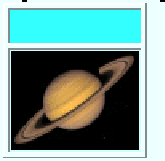
By clicking on the image/gif link you may see the associated image, as shown in figure B.1.
For better understanding of the following functions, we use the existing table Planets to make examples.
The function obtains the URI of the long_expression of the BLOB, and returns it in the form of an HTML reference with the ASCII expression embedded in it.
Example:
SELECT HTMLREF (Small_pic, 'MarsPic') FROM Planets
WHERE Serial =4
Depending on the application where the statement was issued, the results will be of the form:
'<a href="http://194.219.34.132:8181/blobxxxxxxxx">MarsPic</a>'for SQL Query Tool
| MarsPic |
for SQL Terminal. By clicking on MarsPic you can see the associated image.
Function IMAGE checks if the long_expression that is the BLOB is indeed an image through examination of the MIMETYPE of the BLOB argument. If not, it returns a DOMAIN ERROR message. Otherwise, it returns a tag of the form
'<img src="xxxx">'", where "xxxx" is the URI of the image BLOB.
An example of a valid MIMETYPE is e.g. image/gif.
Example:
SELECT IMAGE(Small_pic) FROM Planets WHERE Serial=6;
Depending on the application where the statement was issued the results will be of the form:
'<img src="http://194.219.34.132:8181/blobxxxxxxxx">'for SQL Query Tool
Returns the MIMETYPE of the BLOB as a character string.
Example:
SELECT MIMETYPE(Big_pic) FROM Planets where Serial=1;
returns:
'image/jpeg'
We have already seen in section B.9.(BLOBs and the URI function) the usage of URI.
The Unicode version 1.1 and ISO/IEC 10636-1:1993 jointly define a 16 bit character set, UCS-2, which encompasses most of the world's writing systems. Instead of using only one byte (8 bits), the Unicode uses 2 bytes (16 bits), thus enabling a uniform, easy encoding of any language (including Japanese, Korean and Chinese).
Two data types, unicode char and unicode varchar are provided to allow data definition of Unicode data .
Example of a table creation for Unicode data:
CREATE TABLE uni (
Initial_character char(6),
Uni_string unicode varchar(30)
);
The table uni of the above example has two columns: Uni_symbols, which contains a unicode string and Initial_character, which contains the unicode value of the initial symbol of Uni_symbols (in ASCII).
Unicode characters may be inserted in the table in two different ways:
\u) and the entire string
must also be preceded by u.
Example:
INSERT INTO uni VALUES ('00a5', u'\u00a5\u00a4');
INSERT INTO uni VALUES ('00c3', u'\u00c3\u00d4');
INSERT INTO uni VALUES ('00a5', u'\u00a5\u01ab\u00e5');
It is also possible to insert unicode characters in the middle of an ASCII string, as the following example shows:
INSERT INTO uni
VALUES ('A', u'Another character \u01cd');
Of course this is not the easiest way to insert a unicode value, but it will work on both SQL Query Tool and SQL Terminal. It will also work for all types of browsers, in SQL Terminal, regardless of default character sets.
To insert a unicode character string directly, you must use the prefix character w.
Example:
insert into uni (uni_string)
VALUES (w'
![]() ')
')
To write a unicode string, you will have to find the appropriate keys in the keyboard.
Warning about direct unicode insertion
You must keep in mind that some commercial browsers do not support Unicode correctly.
They do not send data in Unicode, but send 8-bit ASCII, encoded in UTF-8, having a
puzzling effect to users who might perceive this as a malfunction of Ovrimos.
Sometimes, the browser displays Unicode characters incorrectly in input fields but sends
them correctly to the database. Sometimes, it does even do that.
Unicode insertion was handled correctly by Microsoft Explorer 4.x version and
by Netscape Navigator 4.6.
The database parameter CHARSET must be set to UTF-8.
Columns with Unicode data may be selected without any special mention to the type of data.
Example:
SELECT * FROM uni;
After the insertions of the previous section, the table displayed will look like the one in figure B.3.
It is possible to match unicode data using predicates with = or LIKE, e.g.
SELECT * FROM uni WHERE uni_symbols LIKE u'\u00a5%';
The above example fetches all rows where the unicode character string starts with 00a5, as shown in figure B.4.
You may also use unicode data directly in string matching.
Example:
SELECT * FROM uni WHERE uni_symbols LIKE w'
![]() %';
%';
SELECT uni_symbols FROM uni
WHERE uni_symbols like w'Ã\%'
The output of such a query will be as shown in figure B.5.
Parameter CHARSET is set when a new database is created. $CHARSET is used by the browser to take the necessary actions for displaying characters. Default is ISO-8859-1 (The Latin character set).
When a CHARSET other than UTF-8 is used, then
When UTF-8 character set is used, then
All of the above are valid for displaying Unicode in SQL Terminal. Although it is possible to insert unicode data from SQL Query Tool, it is not possible to display them as unicode from SQL Query Tool.
Initially, there is only one schema, sys. Thus, all systems tables, see section B.11.2.(System Tables) are qualified by sys, e.g. sys.users.
There is no explicit schema definition statement in Ovrimos SQL. Every time an object is created, it may potentially be made to belong to any schema. If the object is qualified by a schema name, then the object belongs to this schema.
Example:
CREATE TABLE project1.tab1 (...)
creates a new table tab1, which belongs to schema project1. If project1 does not exist, it is created implicitly and it contains only one object tab1. If project1 already exists, then the new object, is added to the collection of the schema's objects.
If, on the other hand, the table creation statement does not include a schema name, for
example:
CREATE TABLE tab2 (...)
creates a table, which is qualified by the current user's name, who is also the owner of this table.
In other words, all created tables are qualified by a schema name that defaults to the current user name. The user who creates a table is the table owner.
Unqualified tables are visible only by their owners. All other users must use the owner's name to refer to this table.
For example, if table handy is created by user pandora, only pandora may access the table as handy. All other users must accesses is as pandora.handy.
Objects belonging to different schemas may interact, since they belong to the same database. The partitioning is only logical. It does not affect the database workspace.
Tables belonging to different databases cannot interact, since by opening one database the user has access only to objects belonging to that database.
The system tables of Ovrimos are:
It is also possible to see what tables exist in the database, by typing in the statement:
SELECT table_name FROM sys.tables;
To obtain table information data, you may type in the following statement:
SELECT table_name, column_name, type_name
FROM sys.tables a, sys.columns b, sys.data_types c
WHERE a.table_id = b.table.id
   AND b.data_type = c.data_type;
When a database is created, initial users are admin and public. User admin has initial password pegasus and administrator privileges, while user public has NULL password and minimal privileges. User public may not login, since it has no password. It may only be used as a prototype for privilege inheritance.
Warning! You must never update system tables directly through SQL statements. Administrators, wishing to modify user data must always do so from the specifically provided SQL statements. See Create User, Drop User, Update User in section B.4. Supported SQL Statements See also 13.4.5.(Privilege Inheritance).
When a number of update statements is required (i.e. insert, delete, update), all these statements can be grouped together and included between the begin - end delimiters. So, all the statements are sent together for execution after clicking on the Execute button. You also need to add a semicolon (;) at the end of each statement.
   BEGIN;
   INSERT INTO P (P#, PNAME, CITY, PHONE)
   VALUES (1301, 'Hanes', 'London', '83456');
   ..........
   DELETE FROM SP
   WHERE CURRENT OF X;
   .........
   UPDATE P
   SET COLOR='Red'
   WHERE P.COLOR='Green';
   .........
   END;
The above is an example of a Bulk Update. All the updates are propagated to the database after the END statement.

![\includegraphics[width=6cm]{uni1}](img61.gif)
![\includegraphics[width=5cm]{uni2}](img62.gif)
![\includegraphics[width=4cm]{uni3}](img63.gif)